Yes, one more article about R1CS
08 Oct 2024When we describe any proving system we are basically operating on the concepts of “witness” (or “private input”), “public input” (or “public parameters”) and “constraints”. Constraints is a set of conditions that must be met by a witness in a couple with public input to produce a valid proof.
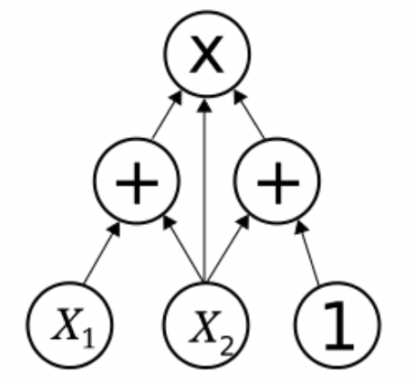
Usually to describe how constraints are combined (mathematically) with inputs we are using arithmetic circuits. Arithmetic circuit is an acyclic graph that consists of an “input”-vertexes and an “action”-vertexes (also called “ gates”). Each “input”-vertex contains an input value and a direction where it should be applied. On the other hand each gate contains a set of input edges (usually two), a set of output edges (usually zero or one) and an operation to be applied to the inputs. The result of this operation is directed by an output edge if exists.
Next we are going to describe the constraint system by using the vector spaces, matrices, their properties and operations, in particular - inner product: \(\langle \mathbf{a}, \mathbf{b}\rangle = \sum a_i\cdot b_i\).
R1CS (Rank-1 constrain system) is a way to describe constraints and how they are applied to the witness and the public input. It has the following form: \(\langle \mathbf{a}, \mathbf{w} \rangle \cdot \langle\mathbf{b}, \mathbf{w}\rangle = \langle\mathbf{c}, \mathbf{w}\rangle\), where \(\mathbf{a}, \mathbf{b}, \mathbf{c}\) is a public vectors that determines the linear combinations of our witness.
Let’s examine several self-describing examples of the simple R1CS circuits.
Simplest circuit
The simplest circuit consist of the only one multiplication gate: \(r = x_1\cdot x_2\). The witness then consists of three values \(\mathbf{w} = (r, x_1, x_2)\) and it has to satisfy our R1CS equation. Then, the tuple \(\mathbf{a}, \mathbf{b}, \mathbf{c}\) is obvious: \(\mathbf{a} = (0, 1, 0), \mathbf{b} = (0, 0, 1)\) and \(\mathbf{c} = (1, 0, 0)\).
Hints
More complex circuits require us to examine several hits:
- Boolean check: if we are using the input value that has to represent a boolean [equals to 1 (true) or to 0 (false)] then we should provide a corresponding check to restrict putting any arbitrary value instead of boolean. This can be achieved by including a simple check that \(x \cdot (x - 1) = 0\) or \(x \cdot x = x\).
- Conditional statement: if our circuit contains a conditional statement that affects the execution flow - we can combine both calculation branches by putting \(x * f_{true}(\mathbf{x}) + (1 - x) * f_{false}(\mathbf{x})\).
- Most circuits require the usage of constants in linear combinations that allows us multiplication by a constant or a constant addition. By putting \(1\) into witness we can achieve any constant by manipulating the coefficients in \(\mathbf{a}, \mathbf{b}, \mathbf{c}\).
More complex circuit
Let’s examine the following procedure:
def r(x1,x2,x3):
  if x1:
    return x2 * x3
  else:
    return x2 + x3
According to the hints described above, it can be represented as \(r = x_1 \cdot (x_2 \cdot x_3) + (1 - x_1) \cdot ( x_2 + x_3)\). Also, we have to add the check for \(x_1\) boolean properties, so the final constraints can be expressed as follows:
- \(x_1 \cdot x_1 = x_1\) (binary check)
- \(A = x_2 \cdot x_3\) (multiplication for “true” branch)
- \(B = x_1 \cdot A\) (selected “true” branch)
- \((1 - x_1) \cdot (x_2 + x_3) = r - B\) (final equation)
These constraints have to be encoded into the R1CS equation with the witness \(\mathbf{w} = (1, r, x_1, x_2, x_3, A, B)\).
The resulting \(\mathbf{a}, \mathbf{b}, \mathbf{c}\) for each of our four constraints are:
| constraint | a | b | c |
|---|---|---|---|
| 1 (binary check) | (0, 0, 1, 0, 0, 0, 0) | (0, 0, 1, 0, 0, 0, 0) | (0, 0, 1, 0, 0, 0, 0) |
| 2 (multiplication for “true” branch) | (0, 0, 0, 1, 0, 0, 0) | (0, 0, 0, 0, 1, 0, 0) | (0, 0, 0, 0, 0, 1, 0) |
| 3 (selected “true” branch) | (0, 0, 1, 0, 0, 0, 0) | (0, 0, 0, 0, 0, 1, 0) | (0, 0, 0, 0, 0, 0, 1) |
| 4 (final equation) | (1, 0, −1, 0, 0, 0, 0) | (0, 0, 0, 1, 1, 0, 0) | (0, 1, 0, 0, 0, 0, −1) |
These separate R1CS constraints can be put together into the 4-dimensional matrix to represent one equation.
Why Rank-1?
You can search for the proof that each R1CS equation can be represented using special matrix, that equals to the outer product of vectors \(\mathbf{a}, \mathbf{b}\) and this matrix rank will be \(1\) (which means that each column/row can be represented by other column/row by multiplying on a certain constant).