File download:
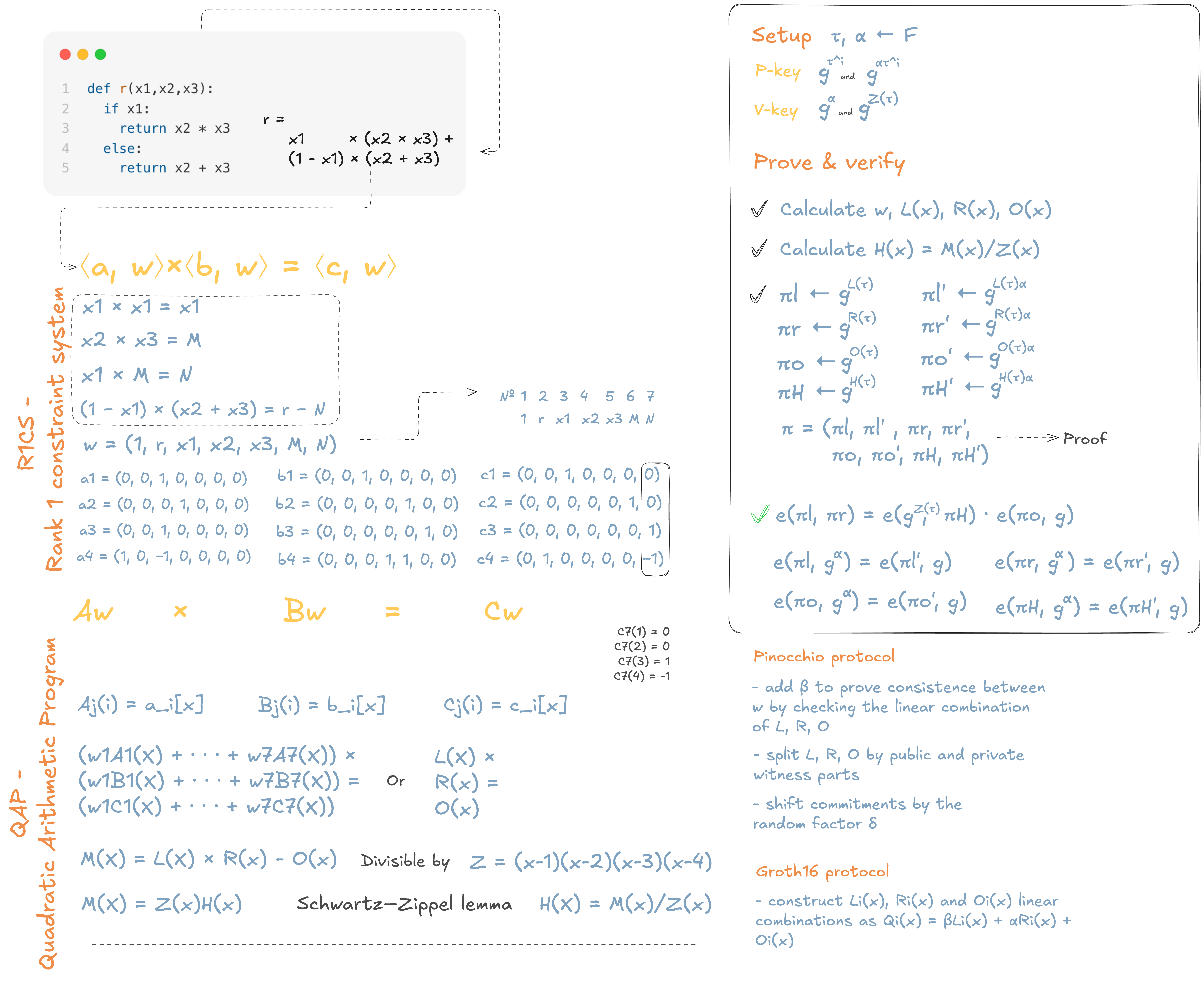
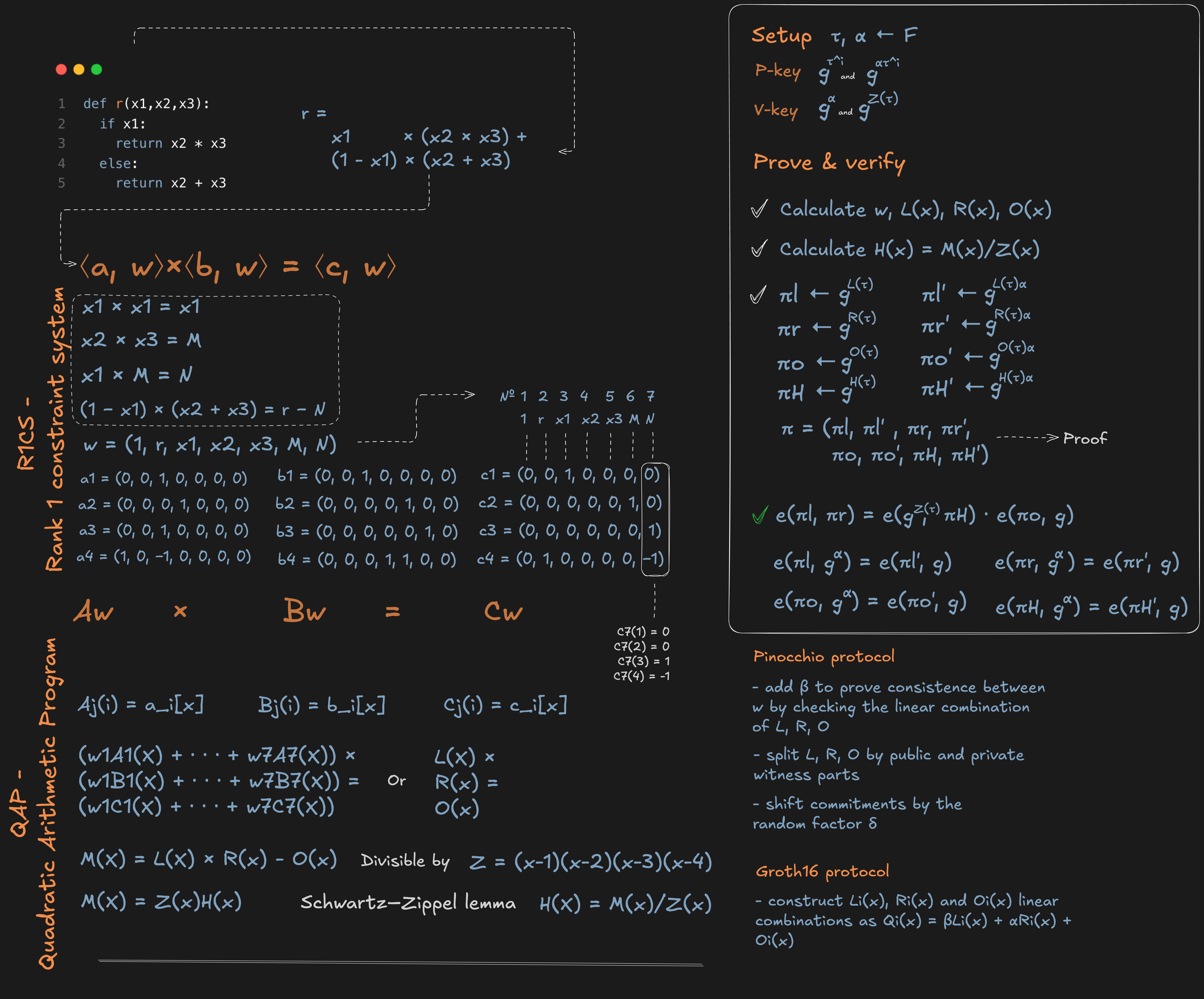
Here, I’m not going to describe the general definition of a zk-SNARK or any related terms. Instead, I’ll try to help the reader understand the underlying math of one of the first popular and novel zk-SNARK protocols, called the Pinocchio protocol, which appeared in 2013.
Special thanks to Anton Levochko and ZK-DL lectures (zkdl-camp.github.io) for the base material for this post.
R1CS
When we describe any proving system, we are basically operating on the concepts of “witness” (or “private input”), “public input” (or “public parameters”), and “constraints.” Constraints are a set of conditions that must be met by a witness coupled with public input to produce a valid proof.
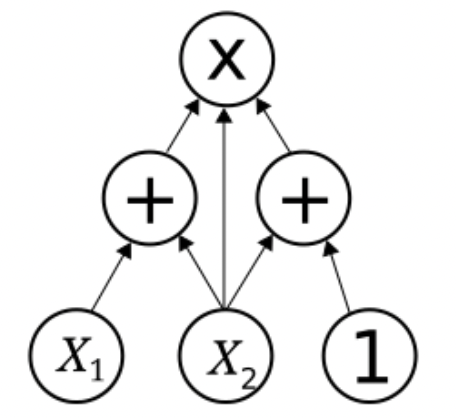
Usually, to describe how constraints are combined (mathematically) with inputs, we use arithmetic circuits. An arithmetic circuit is an acyclic graph that consists of “input” vertices and “action” vertices (also called “ gates”). Each “input” vertex contains an input value and a direction where it should be applied. On the other hand, each gate contains a set of input edges (usually two), a set of output edges (usually zero or one), and an operation to be applied to the inputs. The result of this operation is directed by an output edge if one exists.
Next we are going to describe the constraint system by using the vector spaces, matrices, their properties and operations, in particular, the inner product: $\langle \mathbf{a}, \mathbf{b}\rangle = \sum a_i\cdot b_i$.
R1CS (Rank-1 constraint system) is a way to describe constraints and how they are applied to the witness and the public input. It has the following form: $\langle \mathbf{a}, \mathbf{w} \rangle \cdot \langle\mathbf{b}, \mathbf{w}\rangle = \langle\mathbf{c}, \mathbf{w}\rangle$, where $\mathbf{a}, \mathbf{b}, \mathbf{c}$ are public vectors that determine the linear combinations of our witness.
Let’s examine several self-describing examples of the simple R1CS circuits.
Simplest circuit
The simplest circuit consists of only one multiplication gate: $r = x_1\cdot x_2$. The witness then consists of three values $\mathbf{w} = (r, x_1, x_2)$ and it has to satisfy our R1CS equation. Then, the tuple $\mathbf{a}, \mathbf{b}, \mathbf{c}$ is obvious: $\mathbf{a} = (0, 1, 0), \mathbf{b} = (0, 0, 1)$ and $\mathbf{c} = (1, 0, 0)$.
More complex circuits require us to examine several hints:
- Boolean check: if we are using an input value that has to represent a Boolean [equal to 1 (true) or 0 (false)], then we should provide a corresponding check to restrict putting any arbitrary value instead of a Boolean. This can be achieved by including a simple check that $x \cdot (x - 1) = 0$ or $x \cdot x = x$.
- Conditional statement: if our circuit contains a conditional statement that affects the execution flow, we can combine both calculation branches by putting $x * f_{true}(\mathbf{x}) + (1 - x) * f_{false}(\mathbf{x})$.
- Most circuits require the use of constants in linear combinations that allow us to multiply by a constant or add a constant. By putting $1$ into the witness, we can achieve any constant by manipulating the coefficients in $\mathbf{a}, \mathbf{b}, \mathbf{c}$.
More complex circuit
Let’s examine the following procedure:
def r(x1,x2,x3):
  if x1:
    return x2 * x3
  else:
    return x2 + x3
According to the hints described above, it can be represented as $r = x_1 \cdot (x_2 \cdot x_3) + (1 - x_1) \cdot ( x_2 + x_3)$. Also, we have to add the check for the Boolean properties of $x_1$, so the final constraints can be expressed as follows:
- $x_1 \cdot x_1 = x_1$ (binary check)
- $A = x_2 \cdot x_3$ (multiplication for “true” branch)
- $B = x_1 \cdot A$ (selected “true” branch)
- $(1 - x_1) \cdot (x_2 + x_3) = r - B$ (final equation)
These constraints have to be encoded into the R1CS equation with the witness $\mathbf{w} = (1, r, x_1, x_2, x_3, A, B)$.
The resulting $\mathbf{a}, \mathbf{b}, \mathbf{c}$ for each of our four constraints are:
| constraint | a | b | c |
|---|---|---|---|
| 1 (binary check) | (0, 0, 1, 0, 0, 0, 0) | (0, 0, 1, 0, 0, 0, 0) | (0, 0, 1, 0, 0, 0, 0) |
| 2 (multiplication for “true” branch) | (0, 0, 0, 1, 0, 0, 0) | (0, 0, 0, 0, 1, 0, 0) | (0, 0, 0, 0, 0, 1, 0) |
| 3 (selected “true” branch) | (0, 0, 1, 0, 0, 0, 0) | (0, 0, 0, 0, 0, 1, 0) | (0, 0, 0, 0, 0, 0, 1) |
| 4 (final equation) | (1, 0, −1, 0, 0, 0, 0) | (0, 0, 0, 1, 1, 0, 0) | (0, 1, 0, 0, 0, 0, −1) |
These separate R1CS constraints can be put together into a four-dimensional matrix to represent one equation.
Why Rank-1?
You can search for the proof that each R1CS equation can be represented using a special matrix that equals the outer product of vectors $\mathbf{a}, \mathbf{b}$, and this matrix’s rank will be $1$ (which means that each column/row can be represented by another column/row by multiplying by a certain constant).
QAP
So, above, we described an approach to characterizing the polynomial constraints in the R1CS form: $\langle \mathbf{a}, \mathbf{w} \rangle \cdot \langle\mathbf{b}, \mathbf{w}\rangle = \langle\mathbf{c}, \mathbf{w}\rangle$, where one constraint is represented by public $\mathbf{a}, \mathbf{b}, \mathbf{c}$ vectors. In the example with a more complex circuit, we’ve generated 4 constraints, so we will have 4 tuples of vectors— each tuple for its corresponding constraint. Of course, it seems to be very difficult to prove big circuits using only R1CS - that is why we may want to build a more efficient system based on R1CS. This system is called a Quadratic Arithmetic Program (QAP).
At the beginning, we should recheck our note in the previous post, where I mentioned that we can combine all tuples $\mathbf{a}, \mathbf{b}, \mathbf{c}$ into the corresponding matrices $A, B, C$ and represent our final R1CS circuit as: $A\mathbf{w} + B\mathbf{w} = C\mathbf{w}$. Then, for each column $j$ (that corresponds to the witness’s $j$-th value), we want to build a polynomial $p_j(X)$ where, for each constraint $i \in {1, 2,…}$, $p_j(i)$ is equal to the corresponding $j$-th witness element coefficient in the constraint $i$. This can be done using any appropriate interpolation method (and not only on $X \in {1, 2,…}$ - we can use any fixed set of indexed values for interpolation if the corresponding algorithm requires it). Then, receiving polynomials $A_i(X), B_i(X), C_i(X)$ for each column of the $A, B, C$ matrices, we can rewrite our R1CS as: $(w_1A_1(X) + … + w_nA_n(X)) \cdot (w_1B_1(X) + … + w_nB_n(X)) = $ $(w_1C_1(X) + … + w_nC_n(X))$ evaluated on the $X \in {1, 2,…}$ domain.
Let’s rename the parts of this equation as: $A(X) =(w_1A_1(X) + … + w_nA_n(X))$, $B(X) =(w_1B_1(X) + … + w_nB_n( x))$, $C(X) =(w_1C_1(X) + … + w_nC_n(X))$. Then, our R1CS will have form of $A(X) + B(X) = C(X)$.
We can mention that $A(X) + B(X) - C(X)$ equals some polynomial $M(X)$ that has zeros in $X \in {1, 2,…}$. To convince the verifier that we know such a polynomial with corresponding zeros, we can use the popular principle of proving knowledge of such a polynomial $H(X) = \frac{M(X)}{Z(X)}$ (where $Z(X) = \prod (X - i)$ is known to everyone) by proving knowledge of such polynomials that satisfy the equation $AB - C = HZ$.
The proving algorithm for this relation relies on the Schwartz–Zippel lemma: for a polynomial $P \in F[x]$ of degree $d$ and a uniformly selected $t \in F$, the probability of $P(t) = 0$ is equal to $\frac{d}{|F|}$.
This lemma becomes very useful when we want to prove the knowledge of a polynomial by evaluating it at a random point. If this evaluation can be equal to zero, such a proving system does not make any sense, but when the probability of such an event is small enough, the verifier can be sure that the evaluation is correct.
So, we consider the following protocol:
- The prover shares the coefficients of $H(X)$, named $\mathbf{h} = (h_0, h_1, … h_{n-1})$.
- The verifier selects a random $\gamma$ and sends $\mathbf{\gamma} = (\gamma^0, \gamma^1, … \gamma^{n-1})$.
- The prover responds with the following values: $\pi_A = A(\gamma), \pi_B = B(\gamma), \pi_C = C(\gamma), \pi_M = Z( \gamma) \cdot \langle \mathbf{\gamma}, \mathbf{h}\rangle$.
- The verifier accepts if $\pi_A\pi_B - \pi_C = \pi_M$.
Okay, this protocol follows the correctness property, but how about soundness and zero-knowledge? The proof values queried by the verifier open lots of information about the witness, because the interpolated polynomials over the witness coefficient columns are public and can be calculated by everyone. To deal with this problem, we move to the next protocol, called Proof of exponent.
Proof of exponent
Imagine we have a polynomial $p(x)$, and we want to convince the verifier that it is divisible by another public polynomial $t(x)$. Then, we consider the following protocol: the verifier shares powers of tau ${g^{\tau^i}}$ for some generator $g$—securely generated powers of a randomly selected $\tau$ such that nobody knows $\tau$ itself. Then, the prover calculates the polynomial encryption for $p(x)$ in the following way: $g^{p(\tau)} = \sum (g^{\tau^i})^{a_i}$, where $a_i$ are the coefficients of $p(x)$. The same is done for $h(\tau) = \frac{p( \tau)}{t(\tau)}$. The verifier checks that $g^{p(\tau)} = (g^{h(\tau)})^{t(\tau)}$.
Unfortunately, it is not enough to achieve the soundness property—the prover can still manipulate values of $h(\tau) = r$ to produce a valid proof where $g^{r \cdot t(\tau)} = (g^r)^{t(\tau)}$. That is why we should add “shifted” evaluation of our polynomials by some randomly selected $\alpha$ (in the same way as powers of tau): the verifier additionally shares $g^{\alpha\cdot\tau^i}$ with the prover, and the prover adds to the response the shifted polynomial encryption $g^{p( \alpha\tau)}$. Then, the verifier adds a check for $g^{p(\alpha\tau)} = (g^{p(\tau)})^\alpha$. While the raw values of $\alpha$ and $\tau$ are not accessible to the prover, we achieve the soundness property.
Unfortunately (x2), we still have not achieved zero-knowledge. Because $\tau$ and $\alpha$ seem to be generated by the verifier, we should additionally add our “own shifts” to hide our polynomials in case the $\tau$ and $\alpha$ setup is compromised. It’s actually quite simple: during the proving phase we select random $\delta$ and additionally multiply all our polynomials by it (share $g^{\delta p(\alpha\tau)}$ instead of $g^{p(\alpha\tau)}$ and the same for other polynomial encryptions). While still verifiable, it perfectly hides all information about the polynomials, even if the raw values of $\tau$ or $\alpha$ are known by somebody.